| |
This exercise requires you
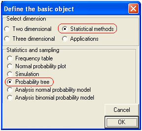
to set the difficulty level to high (in the configuration window). Geocadabra
offers a few nice applications when it comes to probability. This demo
allows for a limited probability tree to be drawn.
We are about to solve the following problem.
A vase is filled with 2 red and 8 blue balls.
After you have paid € 1,25 you are allowed to pick two balls in one go.
Eyes closed of course!You get paid € 3,- for every red ball and nothing
for every blue ball you pick. Do you expect your chances of winning to
increase or decrease depending on the number of turns?
Analysis of the model.
What we are dealing with is a draw without replacement from a vase
containing 2 red and 8 blue balls.
A probability tree will help us list all possible draws in one chart. By
processing this probability tree and by determining the expected value of
the turn out you get an impression of whether you will get paid more or
less than your original stake. |
| |
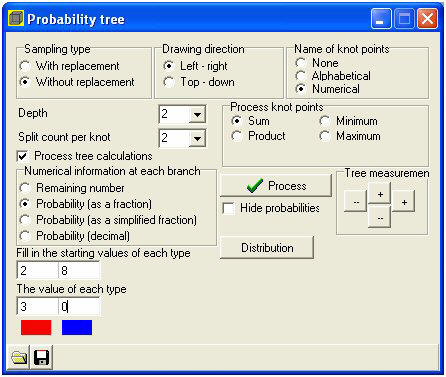 |
Mind the details:
 The sampling type should be without
replacement
Name of knot points: numerical.
After all, we wish to calculate using
amounts.
Depth: 2;
We will take 2 balls from the vase
Split count per knot: 2.
You can either pick a blue or a red
ball so there are 2 possibilities per
ball
Process knot points: sum;
Every red ball is linked to € 3,- and
every blue ball to € 0,- and it is
these amounts you wish to
calculate with.
Numerical information at each
branch: probability (as a fraction)
Starting values of each type:
2 (red) and 8 (blue). |
Value of each type: € 3,- for the red ball and € 0,- for the blue ball
You can click on the red or the blue square to select a colour. In
this example the colours have already
been set.
|
|
Now click the [process]
button. The tree is drawn.
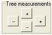
Sometimes the texts in the graph right from the tree are off screen.
Click the buttons where it says “tree measurements” to adjust
the size of the tree horizontally or vertically.
|
|
|
The tree will look like
below:
If you were to, for
example, follow the top branch you would get the following
information:The probability of getting two red balls equals
 .
The sum of the total turnout (€ 3,- per red ball) equals € 6,-. .
The sum of the total turnout (€ 3,- per red ball) equals € 6,-. |
|
|
Now
that the tree has been drawn and processed a new button

has appeared. Click it and a box will appear reading the continuation
computations.
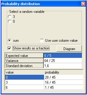
Now select:
Variable: sum
After all, you would like to know the way the fraction functions
Show results as a fraction: select
You would rather not deal with decimals.
The bottom three lines
show the sum’s probability distributions. The bottom line tells
you that the chance to receive a € 6,- turnout equals
 . This is the . This is the
 of the
probability tree. of the
probability tree. |
|
The probability of
receiving € 3,- equals
 . This is the sum
of the turnouts of the two branches that both . This is the sum
of the turnouts of the two branches that both
generate € 3,-. You can now start interpreting this probability
distribution:Out of every 45 times you enter
the draw you will once receive € 6,-, 16 times € 3,- and 28 times
you will receive nothing at all. This comes down to
 euro a turn so
that is an average of € 1,20. Since you have to pay € 1,25 to
enter the draw you will eventually loose € 0,05 every time you
enter. euro a turn so
that is an average of € 1,20. Since you have to pay € 1,25 to
enter the draw you will eventually loose € 0,05 every time you
enter.
|
Epilogue
Geocadabra can calculate models of probability that can be
simulated by means of a draw from a vase with or without
replacement. The number of balls that can be drawn is adjustable
and the same applies to individual colours. However, the maximum
of adjustable colours is limited to 10. Instead of working with
colours you can also work with related figures as is shown in the
turnout above. It is also possible to work with variables (or
stochastic models) per colour or you can work with the sum, the
product or even with the maximum or minimum of the drawn numbers.
You can save a model of probability to continue working on it at a
later date. |
The probability
distribution screen has a button called 
Pressing this will result in a histogram (= vertical bar graph) of
the current probability distribution and this graph can then be
further investigated. You can use a boxplot or you can use the
normal distribution (including expected value and standard
deviation both equal to those of the probability distribution). In
return, you can use these to investigate whether a vase model more
or less meets the characteristics of a normally distributed model.
You can even have the probability distribution drawn out on
regular probability plotting paper. According to the theory this
should result in a straight line when using an exact normal model.
You can now use the rules of thumb as they apply to a normally
distributed model. Alongside is an impression of the model above
but things do not start becoming truly interesting until you start
with a model that has more depth (and colours).
This program will help you support a wonderful learning curve
right to the final levels of secondary education. |
|
|
|
|